The first principle is that you must not fool yourself and you are the easiest person to fool. -Richard P. FeynmanHave you ever fooled yourself? Maybe a better question is, do you remember the last time you fooled yourself? You've worked all day or all week on a problem, and you think you've come up with a reasonable, if not elegant, solution. You show it to someone you trust—a coworker or a friend maybe—and she immediately sees the flaw in your logic or proposes a dead simple alternative that you never thought of. Face-palm.
I fool myself all the time, and I'm not ashamed to admit it. Those face-palms are the times when real learning happens, if you're willing to examine where you went off track and why the better solution works. Then you can generalize it to other problems. I came across one fascinating post by Ivan Yurchenko a few months back that perfectly illustrates how you can fool yourself on multiple levels when you're excited about something and want it to be more than it is.
The post is about calculating the Nth Fibonacci Number in O(log n) time, and it caught my attention because I thought that was impossible. To be clear, I don't want anyone to think I'm trying to take down Ivan or his post in any way. That's not the intent here. I enjoyed reading his post, and it made me think hard about algorithms, benchmarking, and optimization. It's a great post to learn from, and I'm sharing some of the insights I had. Getting back to Fibonacci Numbers, why did the claim of O(log n) time bother me?
Question Your Assumptions
The Fibonacci Numbers are a common sequence of numbers that are generated by starting with 0 and 1 (or 1 and 1, depending on context and personal preference) and continually adding the last two numbers to get the next number in the sequence. The first 10 Fibonacci Numbers are
0, 1, 1, 2, 3, 5, 8, 13, 21, 34, ...Using a loop, we can write a simple program that calculates the Nth Fibonacci Number. Ivan does this, and here is his version in Python:
class IterationFibonacci:
  def __init__(self):
    pass

  def get_number(self, n):
  """Get nth Fibonacci number (n is int, non-negative)."""

    if n == 0:
      return 0
    a = 0
    b = 1
    c = 1
    for i in range(n-1):
      c = a + b
      a = b
      b = c
    return c
where

is the golden ratio, and
Normally, a closed form expression signals that we can compute a result in constant time, but take a closer look at that expression. The n for the Nth Fibonacci Number that we're trying to find is an exponent in two places, and φ and ψ are irrational numbers. Taking the nth power of a number requires n-1 multiplications. That makes the time complexity of this closed-form expression O(n). We could be smarter about the multiplications and split them up into a binary tree of multiplications. That would make the time complexity O(log n).
Can we do better? How about using a power function provided by a standard library? It turns out that the run time complexity of a power function is dependent on the precision that you need in the result, and once you start looking at the precision that you need for Fibonacci Numbers, you start to see the real problem that we're dealing with. The Nth Fibonacci Number will have on the order of n bits in binary form. The 100th number has 69 bits. The 1,000th number has 694 bits. the 10,000th number has 6,942 bits.
It takes a little while for the series to get going, but after a while every subsequent number requires another bit to calculate and store it. That growth means that a power function needs n bits of precision to compute the Nth Fibonacci Number exactly, so it will have O(n) time complexity, assuming you already know the golden ratio to the required number of bits outright. That's the best we can do. Returning to the simple iterative algorithm above, the addition inside the for loop doesn't take constant time. It takes O(n) time because there are O(n) bits to add together. That was the incorrect assumption we were making, and the algorithm actually has O(n^2) time complexity.
That brings us to the matrix multiplication algorithm that Ivan presented from The Art of Computer Programming. It only has O(log n) complexity if you assume that all multiplies can be done in constant time, but the numbers being multiplied are on the order of O(n) bits long so the complexity is actually O(n log n). Knowing that calculating Fibonacci Numbers means working with ginormous numbers is a good thing to keep in mind when figuring out the complexity of a real implementation. The theory may be making assumptions that can't be met on a physical computer.
Pay Attention to What You're Testing
Moving on from complexity theory to benchmarking, Ivan compared the simple iterative algorithm above to the matrix multiplication algorithm, and the results showed that the run time of the iterative algorithm grew linearly and the matrix multiplication algorithm run time appeared to stay constant. There were a couple wrinkles in his tests, though.
The test procedure consisted of doing test runs of each algorithm, calculating 10,000 Fibonacci Numbers around n where n was chosen pseudo-randomly in the range n±5. He did these 10,000-iteration runs over the range of n from 10 to 1010 in increments of 10. Here's the code:
def benchmark():
  random.seed()

  for around in range(10, 1010, 10):
    ifib = IterationFibonacci()
    mfib = MatrixFibonacci()
    ti = 0
    tm = 0
    count = 10000
    for _ in range(count):
      n = random.randint(around-5, around+5)
      t = time.time()
      ifib.get_number(n)
      t1 = time.time() - t
      ti += t1

      t = time.time()
      mfib.get_number(n)
      t2 = time.time() - t
      tm += t2

print("{0}\t{1}\t{2}".format(around, ti, tm))The second issue arises when we look at how the matrix algorithm is implemented. Another optimization was added to the matrix algorithm to speed it up more. In the part of the algorithm that decomposes n into powers of 2 and calculates the matrices for those powers of 2, the matrices are calculated once and saved in a hash table so that they can be recalled the next time they're needed instead of calculating them again. This optimization is called memoization, and it muddies the waters a bit because we're no longer comparing two algorithms, we're comparing one algorithm without an optimization and another one with an optimization. Here's the matrix algorithm with memoization:
class MatrixFibonacci:
    A = [[1, 1],
         [1, 0]]

    def __init__(self):
        self.__memo = {}

    def __multiply_matrices(self, M1, M2):
        """2x2 matrices multiplication"""

        a11 = M1[0][0]*M2[0][0] + M1[0][1]*M2[1][0]
        a12 = M1[0][0]*M2[0][1] + M1[0][1]*M2[1][1]
        a21 = M1[1][0]*M2[0][0] + M1[1][1]*M2[1][0]
        a22 = M1[1][0]*M2[0][1] + M1[1][1]*M2[1][1]
        r = [[a11, a12], [a21, a22]]
        return r

    def __get_matrix_power(self, M, p):
        """Calculate matrix power (p is a power of 2)"""

        if p == 1:
            return M
        if p in self.__memo:
            return self.__memo[p]
        K = self.__get_matrix_power(M, int(p/2))
        R = self.__multiply_matrices(K, K)
        self.__memo[p] = R
        return R

    def get_number(self, n):
        """Get nth Fibonacci number (n is int, non-negative)."""

        if n == 0:
            return 0
        if n == 1:
            return 1
        # Decompose to powers of 2,
        # i.e. 62 = 2^5 + 2^4 + 2^3 + 2^2 + 2^0 = 32 + 16 + 8 + 4 + 1.
        powers = [int(pow(2, b))
                  for (b, d) in enumerate(reversed(bin(n-1)[2:])) if d == '1']
        # Less pythonic: http://pastebin.com/h8cKDkHX

        matrices = [self.__get_matrix_power(MatrixFibonacci.A, p)
                    for p in powers]
        while len(matrices) > 1:
            M1 = matrices.pop()
            M2 = matrices.pop()
            R = self.__multiply_matrices(M1, M2)
            matrices.append(R)
return matrices[0][0][0]To compare the two algorithms directly, we can remove the memoization from the matrix algorithm. Even so, running up to n=1,000 doesn't show a substantial difference between the two algorithms. To get a better sense of their difference, we can run out to n=10,000, which results in run times like this:

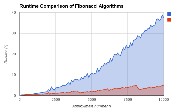
Keep Looking for a Simpler Way
If a solution seems complicated, it probably is. There is often a simpler approach that will accomplish the same goal more clearly and in less code. The above matrix algorithm is pretty complicated, and a few of the commenters on the original post came up with some nice improvements. One that I particularly liked from Juan Lopes was dramatically shorter, and it's reproduced here with a few edits to put it in the same format as the previous algorithms for running in the test bench:
class MatrixFibonacciShort:
  def __init__(self):
    pass

  def mul(self, A, B):
    return (A[0]*B[0] + A[1]*B[2], A[0]*B[1] + A[1]*B[3],
            A[2]*B[0] + A[3]*B[2], A[2]*B[1] + A[3]*B[3])

  def fib(self, n):
    if n==1: return (1, 1, 1, 0)
    A = self.fib(n>>1)
    A = self.mul(A, A)
    if n&1: A = self.mul(A, self.fib(1))
    return A

  def get_number(self, n):
    if n==0: return 0
    return self.fib(n)[1]
I run into this problem all the time where I think long and hard about the best way to express some algorithm only to have someone else (or a Google search) show me a much more elegant solution. It's always great to learn about another clever way to solve a problem, and over time these solutions build up your repertoire. But every time I'm attacking a new problem—and it's good practice to always spend some time reasoning about solutions yourself—I basically assume that whatever solution I come up with, I'll find something better on the internet.
It is so true that the easiest person to fool is yourself, and these mindsets are a good way to prevent at least some foolishness. First, always question your assumptions. Assumptions are the blind spots that hide obvious mistakes. Second, make sure that when you're comparing ideas, you know exactly what you're comparing and you are comparing exactly what you should to reach a valid conclusion. Finally, assume that whatever solution you come up with, a better one exists, especially if your current solution seems too complicated. Then you have to decide if further optimizations are worth pursuing, or if your current solution is good enough.
No comments:
Post a Comment